Shaded Relief Map in Python

Today, we’ll combine different cool stuff: cartopy, Google Maps tiles, SRTM elevation data and shaded relief maps !
We will need cartopy (+ dependencies), which you can install from source, or from C. Gohlke’s prebuilt binaries for Windows users.

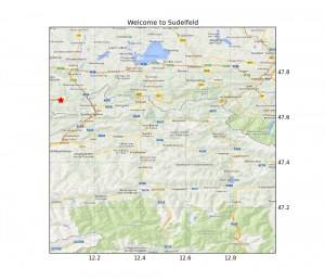
The first map we create will simply show a 1 degree-square zone including Sudelfeld (where I actually am attending “MESS: ObsPy meets Array Processing”). This map will show Google Maps tiles in the background and a small star where the ski resort actually is (see full code for imports needed) :

## Subplot 1: Google Maps Tiles
plt.figure(figsize=(10, 10))
ax = plt.subplot(111, projection=ccrs.PlateCarree())
ax.set_extent([12.0, 13.0, 47.0, 48.0])
gg_tiles = GoogleTiles()
ax.add_image(gg_tiles, 10)

plt.scatter(lon, lat, marker=(5, 1), color='red', s=200)
plt.title("Welcome to Sudelfeld")

this will plot this map:

Next step: get SRTM data automatically using one of cartopy’ many interfaces:

## Subplot 2: STRM Map
plt.figure(figsize=(15, 10))
ax = plt.subplot(111, projection=ccrs.PlateCarree())

elev, crs, extent = srtm_composite(12, 47, 1, 1)
elev = np.ma.masked_less_equal(elev,0,copy=False)
plt.imshow(elev, extent=extent, transform=crs,
           cmap='gist_earth', origin='lower')

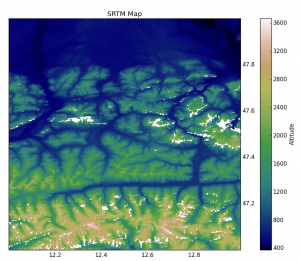
Sadly, there are a lot of gaps in SRTM data for the Alps, so we have to mask the elev array to hide bad values, and the resulting plot is:

To overcome this lack of information, we will use the method described in GDAL’s FillNoData method:

srcband = src_ds.GetRasterBand(1)
dstband = srcband
maskband = srcband
smoothing_iterations = 0
options = []
max_distance = 200
result = gdal.FillNodata(dstband, maskband,
                         max_distance, smoothing_iterations, options,
                         callback=None)
elev = dstband.ReadAsArray()

Apart from a few object tranformation, the core of this function is the maskband for which zero values are considered invalid and non-zero are valid. The max-distance is a threshold for the biggest distance allowed between one invalid point and the closest valid one. The elev array we receive back contains no more gaps :

Step 3: get the slope and aspect of the SRTM data, using numpy.gradient and numpy.arctan/arctan2:

## Subplot 23: Shaded Relief Map
plt.figure(figsize=(10, 10))
ax = plt.subplot(111, projection=ccrs.PlateCarree())
x, y = np.gradient(elev)

slope = np.pi/2. - np.arctan(np.sqrt(x*x + y*y))

# -x here because of pixel orders in the SRTM tile
aspect = np.arctan2(-x, y)

altitude = np.pi / 4.
azimuth = np.pi / 2.

shaded = np.sin(altitude) * np.sin(slope)\
    + np.cos(altitude) * np.cos(slope)\
    * np.cos((azimuth - np.pi/2.) - aspect)

plt.imshow(shaded, extent=extent, transform=crs,
           cmap='Greys', origin='lower')

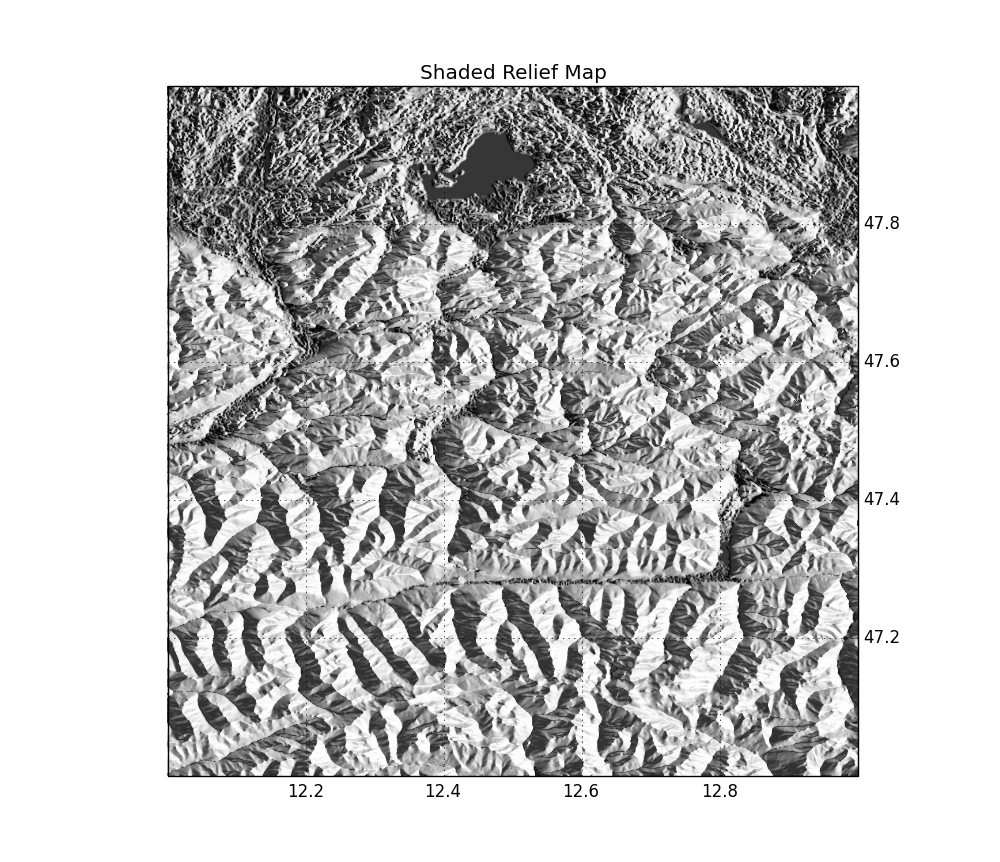
The definition of the shaded variable comes from here, I simply rewrote the processing of the slope and aspect using state of the art numpy routines. For a given azimuth and altitude of the Sun (here it is early morning, Sun on the east), the resulting map looks like:

Done!

From now on, the full-codes will be presented as IPython Notebooks in a GitHub repository and visible using nbviewer