Here is a new tutorial that will include “a bit of all” tutorials previously published on this blog and some new cool stuff to play with !
Idea:
Find some resources on the Internet and plot them on the map of Europe ! In brief: do that:
Step 0: Input Preparation
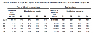
I found some statistics about the preferred period for holidays in the EU, per country (here). On Page 4, you’ll see a table (Table 2) that summarize the number of Tourism Nights spent away by EU residents in 2009, broken down by quaters (right part of the table). The country codes are ISO-like codes, we’ll have to handle that later !
I wanted to have a simple text file to read from the python script, so I copied-paste from the PDF to a text file, merged the big numbers (millions of Germans, for example) and removed the % symbol. Now, the file looks like :
BE 11331 17 25 42 16 84791 12 22 54 12
BG 7861 19 20 43 17 35301 15 19 51 15
CZ 26379 18 26 39 17 119587 14 22 51 13
Etc.
I also needed a file to convert the ISO code to “English Name”, I found the necessary resource on the iso.org website. I saved the file in the same folder.
ARMENIA;AM
ARUBA;AW
AUSTRALIA;AU
AUSTRIA;AT
AZERBAIJAN;AZ
BAHAMAS;BS
BAHRAIN;BH
BANGLADESH;BD
Step 1: Let’s work on the files
I use a new numpy method, called “loadtxt”, which is super easy to work with !
data = np.loadtxt('tutorial06.txt',dtype={'names': ('country', 'N1', 'Q11', 'Q21', 'Q31', 'Q41','N2','Q12', 'Q22', 'Q32', 'Q42'),
 'formats': ('S2', 'i8','i4','i4','i4','i4','i8','i4','i4','i4','i4')})
The data array contains the full table. One can assign the column/row numbers like in any numpy array, or use the field names. It’s important to define dtypes when you have string-type data in a file.
We do the same with the ISO-Country file :
countries = np.loadtxt('list-en1-semic-3.txt',skiprows=2,
 dtype={'names': ('country', 'ISO'),
 'formats': ('S255', 'S2')},
 delimiter=';')
Note, here, we set the “skiprows=2” and “delimiter=;” so the method knows where to start reading, and how to split the lines.
Step 2: Parse data, get the coordinates and plot !
So, for each line in the data array, we will try to get :
- The name of the country
- The coordinates of this country
With this data, we will plot a pie charts of the data, centered on the coordinates.
for di in data:
 iso, N1, Q11, Q21, Q31, Q41, N2, Q12, Q22, Q32, Q42 = di

 #The "eurostat" file contains "non-iso" codes, we need to convert:
 if iso == 'EL': iso='GR'
 elif iso =='UK': iso='GB'

 #We use numpy.ma to find the country name based on the iso code:
 mask = ma.masked_where(countries['ISO'] != iso, countries['ISO'])
 country = ma.array(countries['country'],mask=mask.mask).compressed()[0]

 #Now, let's geolocate the country name using GoogleMaps API:
 country = country.replace(' ','%2F') #needed for GoogleMaps API to recognize the "space"
 request = "http://maps.google.com/maps/geo?output=csv&q=%s" % country
 url_info = urllib2.urlopen(request)
 line = url_info.read()
 url_info.close()
 status, zoom, lat, lon = line.split(',')

 #Projection on the Basemap:
 X, Y = m(float(lon), float(lat))

 # Taking the "Tourism nights in 2009" quarters:
 r1 = Q12/100.
 r2 = Q22/100.
 r3 = Q32/100.
 r4 = Q42/100.

 #Useless print to debug
 print country, iso, lon, lat, r1, r2, r3, r4, r1+r2+r3+r4

 #Calling the draw_pie function (see tutorial05):
 draw_pie(ax,[r1, r2, r3, r4], X, Y,size=200)

 time.sleep(0.4) #Needed because I did not provide my GoogleMaps API key !
The iso code for Greece and Great Britain are not properly set in the EU-data file, so we need to correct them before masking the ISO-array to recover the country name.
Once we have the country name, we can ask GoogleMaps API to give us the coordinates. Here, I do not use the free API key google provides, and I have to set a time.sleep(0.4) (seconds) between two requests, otherwise my requests get trashed.
Using urrlib2, we can ask Google, and read the result of the location.
Finally, we project the (lon, lat) to (X,Y) and plot the pie chart, and… It’s done !!
Conclusions:
Most EU residents tend to go on vacation on Q3 !!
See the full code after the break !
Data file : tutorial06.txt
Data file : list-en-semic-3.txt
#
# BaseMap example by geophysique.be
# tutorial 06

"""
Using :
-- An example makes custom 'pie charts' as the markers for plot Thanks to Manuel Metz for the example
"""

import math
import numpy as np
import matplotlib.pyplot as plt
from mpl_toolkits.basemap import Basemap
import numpy.ma as ma
import urllib2
import time

### PARAMETERS FOR MATPLOTLIB :
import matplotlib as mpl
mpl.rcParams['font.size'] = 10.
mpl.rcParams['font.family'] = 'Comic Sans MS'
mpl.rcParams['axes.labelsize'] = 8.
mpl.rcParams['xtick.labelsize'] = 6.
mpl.rcParams['ytick.labelsize'] = 6.

colors = ['red','blue','green','yellow','magenta','purple','red','blue','green','yellow','magenta','purple']

def draw_pie(ax,ratios=[0.4,0.3,0.3], X=0, Y=0, size = 1000):
 xy = []
 start = 0.
 for ratio in ratios:
 x = [0] + np.cos(np.linspace(2*math.pi*start,2*math.pi*(start+ratio), 30)).tolist()
 y = [0] + np.sin(np.linspace(2*math.pi*start,2*math.pi*(start+ratio), 30)).tolist()
 xy.append(zip(x,y))
 start += ratio

 for i, xyi in enumerate(xy):
 ax.scatter([X],[Y] , marker=(xyi,0), s=size, facecolor=colors[i])

fig = plt.figure(figsize=(11.7,8.3))
#Custom adjust of the subplots
plt.subplots_adjust(left=0.05,right=0.95,top=0.90,bottom=0.05,wspace=0.15,hspace=0.05)
ax = plt.subplot(111)
#Let's create a basemap of Europe
x1 = -20.
x2 = 40.
y1 = 32.
y2 = 64.

m = Basemap(resolution='i',projection='merc', llcrnrlat=y1,urcrnrlat=y2,llcrnrlon=x1,urcrnrlon=x2,lat_ts=(x1+x2)/2)
m.drawcountries(linewidth=0.5)
m.drawcoastlines(linewidth=0.5)
m.drawparallels(np.arange(y1,y2,2.),labels=[1,0,0,0],color='black',dashes=[1,0],labelstyle='+/-',linewidth=0.2) # draw parallels
m.drawmeridians(np.arange(x1,x2,2.),labels=[0,0,0,1],color='black',dashes=[1,0],labelstyle='+/-',linewidth=0.2) # draw meridians

# data is :
## http://epp.eurostat.ec.europa.eu/cache/ITY_OFFPUB/KS-SF-10-054/EN/KS-SF-10-054-EN.PDF page 4:
##  - Table 2: Number of trips and nights spent away by EU residents in 2009, broken down by quarter
##    - Tourism nights (2009) (right part of the table)

data = np.loadtxt('tutorial06.txt',dtype={'names': ('country', 'N1', 'Q11', 'Q21', 'Q31', 'Q41','N2','Q12', 'Q22', 'Q32', 'Q42'),
 'formats': ('S2', 'i8','i4','i4','i4','i4','i8','i4','i4','i4','i4')})

# data is :
## http://www.iso.org/iso/country_codes/iso_3166_code_lists.htm
##  - Text csv version
countries = np.loadtxt('list-en1-semic-3.txt',skiprows=2,
 dtype={'names': ('country', 'ISO'),
 'formats': ('S255', 'S2')},
 delimiter=';')

for di in data:
 iso, N1, Q11, Q21, Q31, Q41, N2, Q12, Q22, Q32, Q42 = di

 #The "eurostat" file contains "non-iso" codes, we need to convert:
 if iso == 'EL': iso='GR'
 elif iso =='UK': iso='GB'

 #We use numpy.ma to find the country name based on the iso code:
 mask = ma.masked_where(countries['ISO'] != iso, countries['ISO'])
 country = ma.array(countries['country'],mask=mask.mask).compressed()[0]

 #Now, let's geolocate the country name using GoogleMaps API:
 country = country.replace(' ','%2F') #needed for GoogleMaps API to recognize the "space"
 request = "http://maps.google.com/maps/geo?output=csv&q=%s" % country
 url_info = urllib2.urlopen(request)
 line = url_info.read()
 url_info.close()
 status, zoom, lat, lon = line.split(',')

 #Projection on the Basemap:
 X, Y = m(float(lon), float(lat))

 # Taking the "Tourism nights in 2009" quarters:
 r1 = Q12/100.
 r2 = Q22/100.
 r3 = Q32/100.
 r4 = Q42/100.

 #Useless print to debug
 print country, iso, lon, lat, r1, r2, r3, r4, r1+r2+r3+r4

 #Calling the draw_pie function (see tutorial05):
 draw_pie(ax,[r1, r2, r3, r4], X, Y,size=200)

 time.sleep(0.4) #Needed because I did not provide my GoogleMaps API key !

plt.savefig('tutorial06.png',dpi=300)
plt.show()
![Number of trips and nights spent away by EU residents in 2009, broken down by quarter [Tourism nights (2009)]](http://www.geophysique.be/wp-content/uploads/2010/11/tutorial06-300x248.png)


